Understanding Apache Spark Query Execution Plans

Arslan Ashraf

March 2024

Credit: this post roughly follows a lecture by senior data engineer at Mckinsey, Afaque Ahmad [1].

In this guide, we will explore some of the basics of Apache Spark's query execution plans. With datasets becoming ever larger, single machine based tools such as Pandas simply don't scale to enormous datasets. We have to move away from a computer, to a cluster of computers.

Spark was designed with the goal of being able to process datasets of enormous size. To build such a system, the creators of Spark built a distributed data processing engine that operates on a cluster of machines performing in-memory parallel processing. Every time we enter the realm of distributed systems, we enter very complicated territory.

What can make Spark challenging to work with is that the data to be processed is stored in multiple machines and sometimes, to process that data, the data has to move around those machines. In Spark, this is called "shuffling". The query execution plan effectively determines how Spark is going to operate on a dataset.

To gain some insight into what Spark is doing under the hood, we will consider two fictional datasets, a customers table and an orders table which we see below respectively. We also see that each dataframe has four partitions. That means the dataset is divided into four parts and each part could be stored in a separate machine.

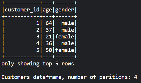
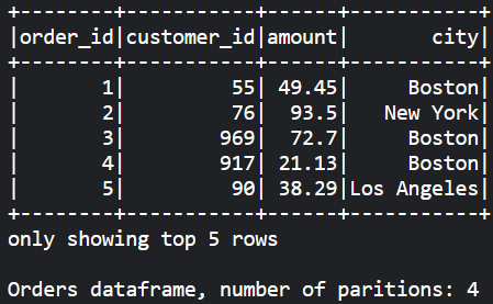
We start by having a look at a rather simple filter operation. We filter the orders dataframe to get transactions that took place in New York.

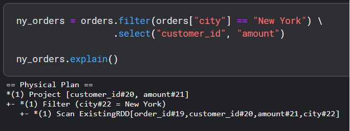
We read the Spark query execution plan from bottom to top. First, there is a scan to read in the dataset followed by a filter operation on the city column with "city#22 = New York". Finally, there is a projection that effectively contains our select function.

Spark by default partitions our dataset and these partitions are spread across worker machines for efficient parallel processing. But what if we wanted to increase or decrease the number of partitions for more efficient processing? We can increase/decrease the number of partitions with the repartition() function.

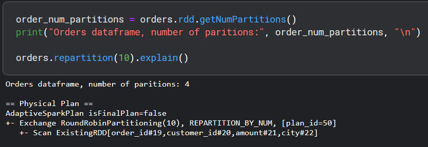
In the second step, Exchange RoundRobinPartitioning(10), REPARTITION_BY_NUM, ..., the term Exchange means Spark is going to do a shuffle or move data around various machines in the Spark cluster. In general, shuffles are a very expensive operation and we want to avoid those.

The term RoundRobinPartitioning(10) means Spark is going to create 10 partitions which we requested and spread the data around in a round-robin fashion. The term REPARTITION_BY_NUM means that Spark will perform the round-robin spreading by row_id_number for each data point to decide which data point is to end up at which partition.

The last step AdaptiveSparkPlan isFinalPlan=false is Spark's internal group of algorithms around "Adaptive Query Execution (AQE)". Spark makes various optimizations based on statistics in the dataset such as number of bytes, partition size, and more. The isFinalPlan=false means that the physical plan in question is not necessarily Spark's final plans but it's generally the same or quite close.

Now to reduce the number of partitions, we can still use repartition(), but there is another more efficient method called coalesce(). The difference is that coalesce() tries to minimize shuffling of the data which is very costly. So let's see coalesce() in action.

In this example, we see that there is not exchange this time, meaning there is no movement of data among the machines and all data in each machine remains only on that machine.

Now let's have a look at the query plan if we join the two dataframes on the "customer_id" column.

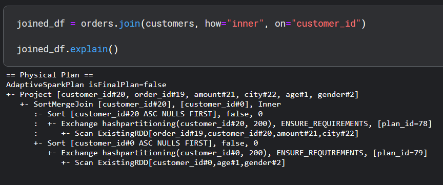
This plan is quite large but we see that there are two groups of similar operations for each dataset. First Spark will scan each dataset, then perform a shuffle in the step Exchange hashpartitioning(customer_id.... In this step, Spark moves data around by applying a hash function to each customer_id and then taking a modulus. This approach ensures that all rows with the same customer_id in the customer dataset and the order dataset end up on the same machine.

Once the data points arrive in their appointed machine, Spark then sorts the data and finally performs a join. The term for this join scheme is "SortMergeJoin". The Project [customer_id#20, order_id#19, amount#21, city#22, age#1, gender#2] term simply selects the listed columns.

Now let's try to understand Spark's query execution plan for a groupby operation.

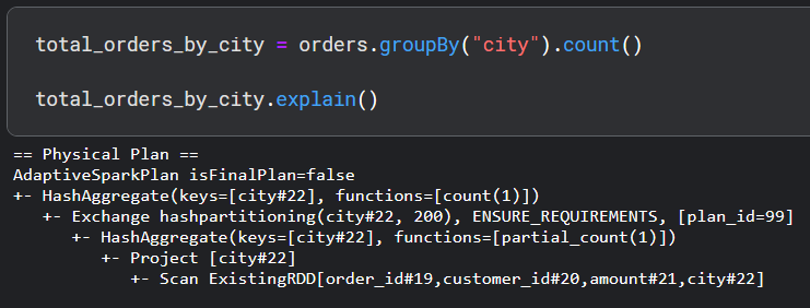
As usual, first, there is a scan to read the data, Spark then does a projection to select the city column. Then there is a HashAggregate(keys=[city#22], functions=[partial_count(1)]) which does a local grouping and count only on the data within each machine. This is shown by functions=[partial_count(1)]. This is an optimization that Spark performs to shuffle less data around machines.

The next step, Exchange hashpartitioning(city...), does a shuffle of a much smaller already aggregated dataset using the hashpartitioning strategy that we discussed earlier. This ensures all the local counts for each unique city column end up in the same machine.

Spark then does another hash aggregate and this time the function functions=[count(1)] is used to get all of the counts.

Finally, let's see a groupby and aggregate operation.

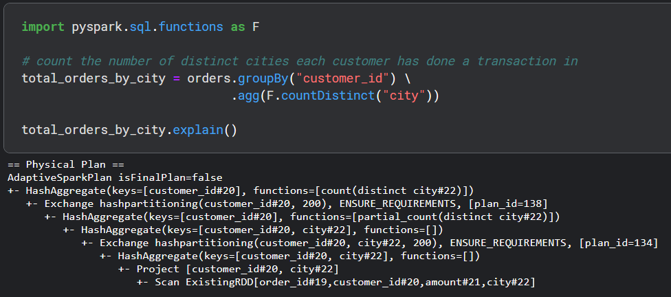
As we can see, there are four hash aggregations and two shuffles happening here. The key thing to note is that first, there is a local aggregation and then there is a global aggregation. After scanning and projection, there is a HashAggregate(keys=[customer_id#20, city#22], functions=[]). Notice that this time the hash aggregation is being done on two keys, customer_id and city. functions=[] means Spark is pulling out only rows that have a distinct pair of customer_id and city. To see this more clearly, Spark takes the following dataset:

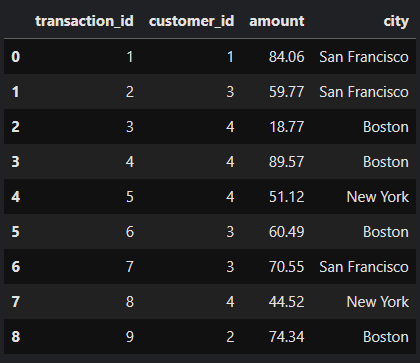
and pulls out all the rows that have a distinct pair of customer_id and city:

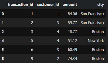
Spark then shuffles this smaller dataset across machines based on the hash of two keys, customer_id and city. This ensures that rows with the same pair of id and city end up in the same machine once the data arrives at its intended destination. The data in one machine or partition after arriving from different machines or partitions may look like this:

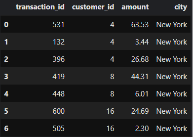
Spark then does two more hash aggregates. The first one, HashAggregate(keys=[customer_id#20, city#22], functions=[]), is actually very much the same as we saw previously. After performing this operation, the data would be filtered as:

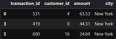
The second hash aggregate, HashAggregate(keys=[customer_id#20], functions=[partial_count(distinct city#22)]), is only on the customer_id and Spark does a partial_count(distinct city).

Now that Spark has the number of distinct city counts for each customer on a local level. Spark needs to do another shuffle to get global distinct counts. Finally, there is one last hash aggregation, HashAggregate(keys=[customer_id#20], functions=[count(distinct city#22)]) and we see that the function applied does a full count distinct on the city column.

References

[1] https://www.youtube.com/watch?v=KnUXztKueMU